When modeling your base case scenario in SC Navigator, the easiest way to define transportation cost is by using a per-unit rate (e.g., per kg or case) for each transport mode. This works well when you have reliable historical data.

However, challenges arise when simulating new scenarios—like serving customers from different warehouses—because cost data for non-existing lanes is often missing. This tutorial shows how to estimate transportation costs using historical data, giving you a per-unit-per-distance cost for each warehouse. This normalized metric helps model alternative distribution strategies quickly and effectively.

1. Starting Point – Required Data

To begin, gather the following data for each warehouse:

• Total demand served by the warehouse in a defined historical period.
• Actual shipment volumes from the warehouse to each customer (Base Case volumes).
• Total transportation cost incurred by the warehouse during that period.

(Note: This cost data should come from your ERP or TMS system, not SC Navigator/AIMMS.)

2. Build Your Baseline Scenario in SC Navigator

Before estimating average costs, you need to create a feasible baseline model that replicates your actual historical flows.
To do this, you must enforce Base Case Volumes in your model. This is explained in the Strategic Network Design e-Learning module.

3. Run the Baseline Scenario

Run the optimization with Base Case Volumes enforced. This ensures the model accurately reflects how goods were actually shipped during the historical period.

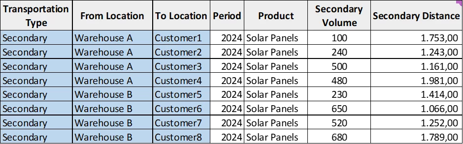
4. Extract Lane Distances

After running the scenario:

1. Go to the Result Details section in the SC Navigator workflow.
2. Open the Transportation Report.
3. Download the lane-level transportation data, including:
   • Volumes per lane
   • Distances per lane (from warehouse to customer)

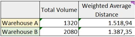
5. Calculate Weighted Average Distance
Using the downloaded table:

• Calculate the weighted average distance from each warehouse to its customers, using shipment volumes as weights.

Steps:

1. Multiply the distance by the volume for each lane.
2. Sum all the resulting values.
3. Divide the total by the sum of all volumes.

This represents the average distance over which a warehouse delivers goods.

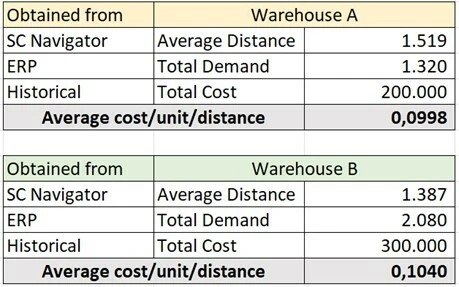
6. Estimate Average Cost per Unit per Distance

Use the following formula:

Average Cost per Unit per Distance = Total Transport Cost / (Total Volume × Weighted Average Distance)

This results in a normalized transportation cost that you can apply to new or hypothetical lanes, even those that weren’t historically used.

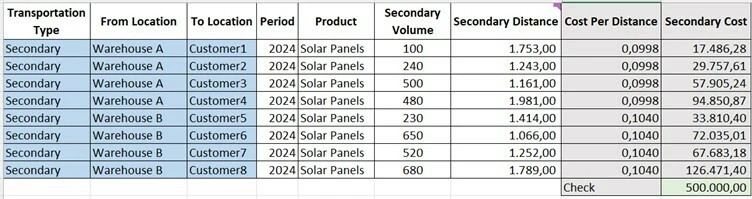
7. Verification Step (Optional but Recommended)

To validate your estimation:

• Recalculate the total cost by applying the average cost per unit per distance to the secondary volume and distance data (from step 4).
• The sum of these estimated lane costs should exactly match the historical total transportation cost from your ERP.

Conclusion

By using this method, you can confidently simulate new potential distribution flows (e.g., serving customers from different warehouses) and assess their feasibility—without needing exact transport cost quotes upfront.

This technique is particularly useful in early-stage network design projects, where flexibility, speed, and reasonable accuracy are more important than absolute precision